LLM & Embeddings — One Predicts Words. One Maps Meaning.
A walk through the two foundational mechanisms behind every modern NLP system — generative language models and similarity-based embeddings — using five hands-on exercises with Hugging Face and Gensim. Week 6 mini-project of the IITM Pravartak Professional Certificate Programme in Agentic AI.
On this page
The model is what writes the email. The embedding is what finds the one you wrote last March.
Most modern AI systems are built from two fundamentally different mechanisms, and most confusion about what AI “is” comes from conflating them. LLMs are generative: tokens in, tokens out, with the output shaped by the prompt and the sampling settings, varying every time you ask. Embeddings are geometric: a deterministic mapping from a word or sentence to a fixed vector, where comparisons are positional and identical input always produces identical output. Both are essential. Both are old enough to be uncontroversial. Most useful systems combine them.
What follows is the Week 6 Graded Mini Project of the IITM Pravartak Professional Certificate Programme in Agentic AI and Applications, used here as a lens for both mechanisms across five hands-on exercises.
The two paths, side by side
The header image above shows the contrast in one frame. The LLM path is a loop with sampling — non-deterministic by design, behaviour controlled by temperature, top-p, and prompt structure. The embedding path is a one-shot lookup followed by a geometric comparison — deterministic, fast, stable.
That single distinction tells you which mechanism to reach for. If the answer needs to be written, generated, synthesized, or improvised, you want the LLM. If the answer needs to be found, ranked, deduplicated, clustered, or routed, you want embeddings. Most production systems use both because most real problems are some combination of “find the right context” and “say something useful about it.”
A quick decision table to anchor the rest of the article:
| Problem | Reach for |
|---|---|
| Semantic search over a corpus | Embeddings |
| Conversational reply or text drafting | LLM |
| Near-duplicate detection or content clustering | Embeddings |
| Summarization of a long document | LLM |
| Routing a support ticket to the right team | Embeddings + a small classifier head |
| Question answering grounded in your docs | Both (RAG) |
| Image or text classification | Embeddings + a categorical head |
| Translation, rewriting, code generation | LLM |
The exercises below show why each row works the way it does.
Exercise 1: Text generation reveals prompt and sampling sensitivity
Section A1 loaded distilgpt2 through the Hugging Face pipeline API and generated three continuations of the same prompt:
generator = pipeline("text-generation", model="distilgpt2")
generator("AI is transforming industries by",
          max_new_tokens=40, num_return_sequences=3, do_sample=True)
Three continuations came back from the same model, the same prompt, the same call:
“AI is transforming industries by using science to bring people together with a greater understanding of the importance of science. The new book takes an approach to both science and technology, allowing people to focus more more effectively on the basics and to…”
“AI is transforming industries by replacing the manufacturing sector with a manufacturing sector that can be turned into a manufacturing and IT sector by creating new jobs and creating new jobs. The new jobs and investment in the next decade will help spur growth…”
“AI is transforming industries by creating a new, faster, and more attractive way of generating capital and creating jobs for both the United States and Europe. This is an effective new way of doing this.”
Three different stories. None of which the model “knew” — it just produced plausible-sounding next tokens under stochastic sampling. Notice the repetitions (“manufacturing sector with a manufacturing sector”), the loops (“more more effectively”), the empty filler (“a new, faster, and more attractive way of generating capital”). DistilGPT-2 is a small model — these are the artefacts of a system that’s good at local fluency but doesn’t have a strong forward plan.
The headline insight: LLM outputs are statistical, prompt-sensitive, and unrepeatable unless you fix the seed. The same prompt can give you variety (a feature when brainstorming) or drift (a bug when consistency matters).
Exercise 2: Tokenization is where the abstraction begins
This is the section to slow down on. Take the sentence:
“LLMs are powerful tools for natural language understanding.”
A human reads eight words. The model sees ten tokens.
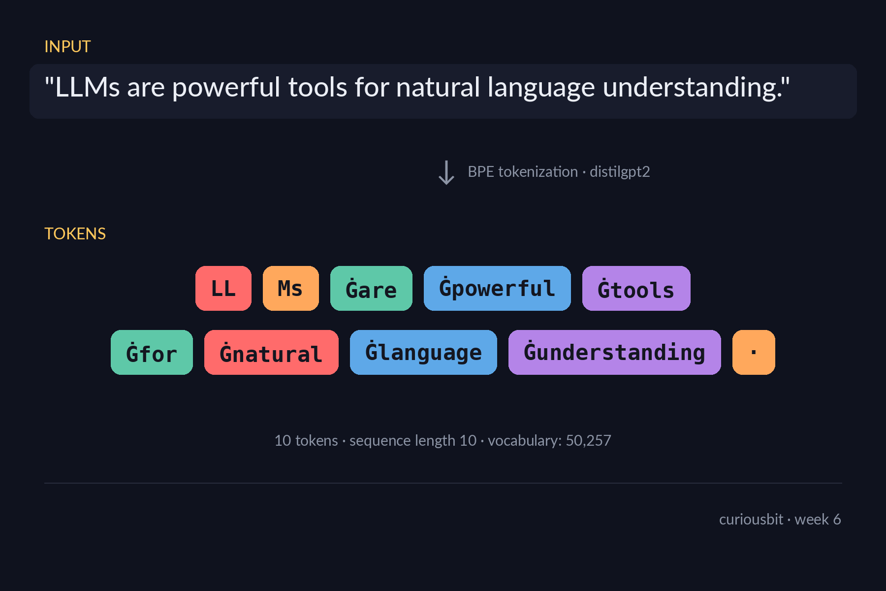
After BPE (Byte-Pair Encoding) with the DistilGPT-2 tokenizer:
['LL', 'Ms', 'Ġare', 'Ġpowerful', 'Ġtools', 'Ġfor', 'Ġnatural',
 'Ġlanguage', 'Ġunderstanding', '.']
The string LLMs doesn’t appear in the model’s vocabulary as a single unit, so it is split into LL and Ms. The Ġ prefix encodes “preceding space” — that’s how BPE preserves word boundaries without a separator character. The period gets its own token.
The mismatch between what a human reads and what the model processes has real consequences:
- Cost is per token, not per word. API billing, latency, and rate limits are all token-denominated. A 1,000-word prompt to a frontier model may bill at 1,300–1,500 tokens depending on language.
- Context windows are token windows. A 4,096-token context holds roughly 3,000 English words. Much less for code (whitespace and symbols inflate counts), much less again for languages with poor vocabulary coverage in the tokenizer.
- Rare strings behave oddly. Brand names, technical acronyms, foreign words, internal jargon — anything outside the trained vocabulary gets fractured. Model behaviour around those fractures is harder to predict, and prompt sensitivity often hides at this layer.
- The same string can tokenize differently with leading whitespace.
"king"and" king"are different token sequences. That’s why pasted prompts sometimes produce subtly different outputs than typed ones.
Tokenization is the lowest layer of the LLM stack and the one most engineering conversations skip. If you’re tuning prompts and getting unstable behaviour, the first place to look is what your input looks like after the tokenizer touches it, not what it looks like in your editor.
Exercise 3: Prompts shape what you get
Section B ran three task-shaped prompts through the same generator, with temperature=0.8 and top_p=0.95:
- Summarization — explicit instruction with a 30-word cap.
- Q&A — structured format with
Q:andA:markers. - Creative — open-ended request for a 4-line poem about AI.
The summarization output respected the spirit of the constraint but drifted past 30 words on most runs — DistilGPT-2 is small enough that hard length control isn’t reliable even with explicit instructions. The Q&A output, asked for the capital of Japan, returned I believe... — the model hedged. A larger model would say Tokyo confidently; a small model produces statistically plausible Q&A-shaped text without strong factual grounding. The creative prompt produced varied and stylistic continuations, but with the lowest grounding: fluency over precision.
Structure compresses the output space the model is sampling from. Vagueness expands it. That single sentence is most of what “prompt engineering” actually is — the rest is technique.
Exercise 4: Word embeddings encode semantic geometry
Pivot to the other mechanism. Section C1 loaded GloVe vectors (glove-wiki-gigaword-50 — 50 dimensions, trained on Wikipedia and Gigaword) via Gensim, then asked for the five nearest neighbours of three words:
| Query | Top 5 neighbours (cosine similarity) |
|---|---|
king | prince (0.82), queen (0.78), ii (0.77), emperor (0.77), son (0.77) |
queen | princess (0.85), lady (0.81), elizabeth (0.79), king (0.78), prince (0.78) |
diamond | gold (0.77), diamonds (0.77), gem (0.74), silver (0.72), jewel (0.71) |
There is no generation here. Each word is mapped to a fixed 50-dimensional vector, and the “nearest neighbours” are the words whose vectors sit closest in that space by cosine similarity. The geometry was learned by training on co-occurrence — words that appear in similar contexts end up in similar positions. That’s why king and prince are nearest neighbours, why queen pulls in elizabeth (the corpus has plenty of references to Queen Elizabeth), and why diamond cleanly resolves to a jewellery cluster.
The classic king − man + woman ≈ queen analogy works in this same space; the lab didn’t run it, but the geometry is there. Embeddings don’t write anything — they place things near other things. That single property is what makes them the backbone of semantic search, retrieval, deduplication, and recommendation.
Exercise 5: Sentence similarity from averaged word vectors
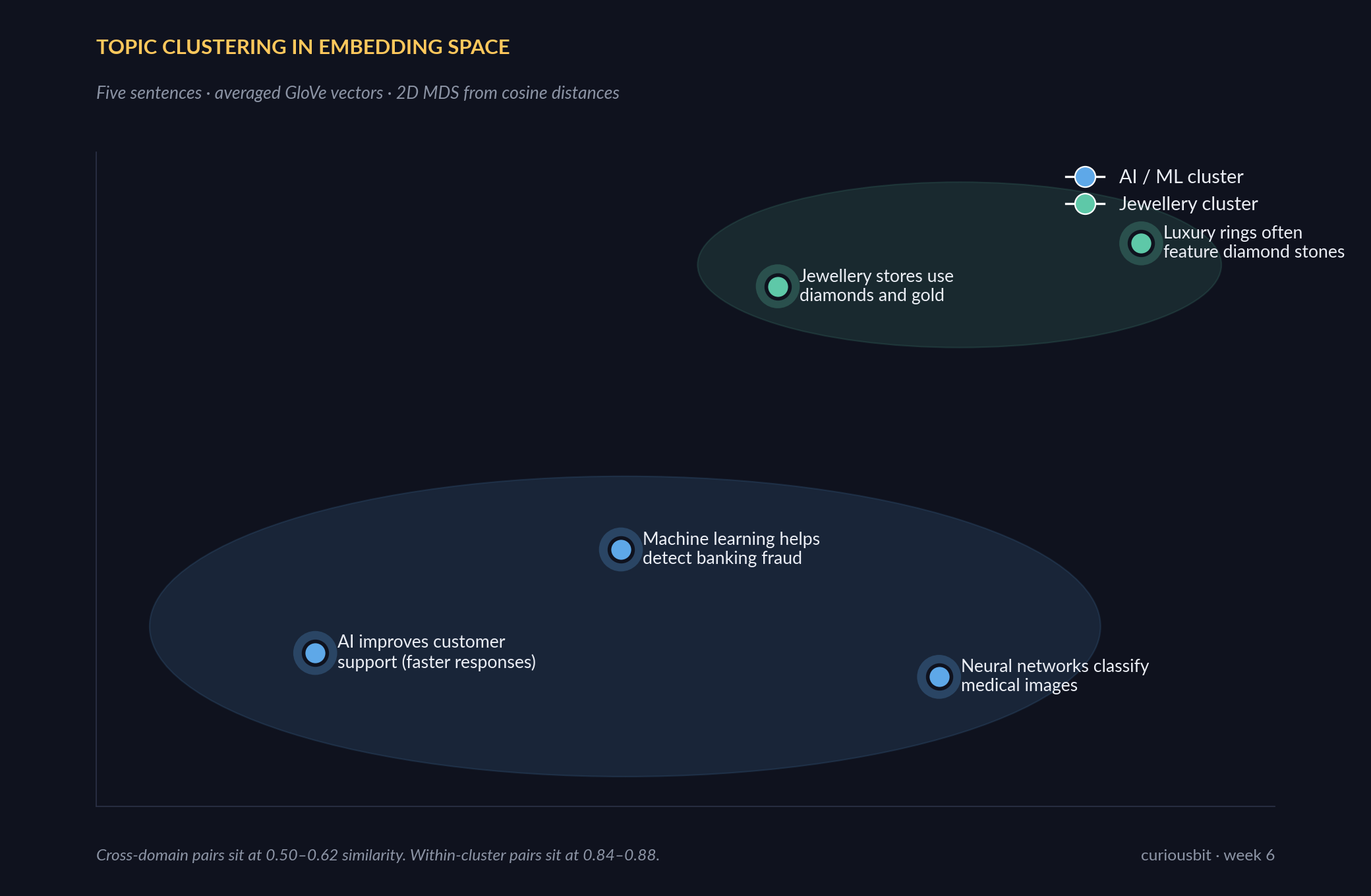
Section C2 extended the geometry to sentences. Five short sentences across two topics — AI/ML and jewellery — were averaged into sentence vectors (mean of their word vectors, with simple lowercase tokenization), then compared with cosine similarity.
Plotted in 2D via multidimensional scaling on the cosine distances, the clustering is unambiguous:
The numerical version:
| AI/support | ML/fraud | Jewellery | Neural/medical | Luxury/rings | |
|---|---|---|---|---|---|
| AI/support | 1.00 | 0.84 | 0.60 | 0.80 | 0.50 |
| ML/fraud | 0.84 | 1.00 | 0.73 | 0.83 | 0.62 |
| Jewellery | 0.60 | 0.73 | 1.00 | 0.58 | 0.88 |
| Neural/medical | 0.80 | 0.83 | 0.58 | 1.00 | 0.56 |
| Luxury/rings | 0.50 | 0.62 | 0.88 | 0.56 | 1.00 |
Within-cluster pairs sit at 0.84–0.88. Cross-domain pairs sit at 0.50–0.62. The grouping is exactly what you’d want a retrieval system to do.
Three caveats worth naming, because they explain why modern retrieval doesn’t actually use GloVe averages:
- Averaging discards word order. “Dog bites man” and “man bites dog” produce identical sentence vectors. For most retrieval that’s tolerable; for anything where syntax carries the meaning, it isn’t.
- Transformer encoders fixed this. Models like BERT, RoBERTa, and their descendants produce contextual embeddings — each token’s vector depends on the tokens around it. Pool those across a sentence and you get a representation that respects word order and disambiguates polysemy.
- Sentence-BERT and friends made it production-grade. SBERT (and successors like OpenAI’s
text-embedding-3, Cohere’s embeddings, Voyage, etc.) trained encoders specifically for sentence-level similarity. That’s the difference between “the demo works on five sentences” and “you can index a million documents and search them in milliseconds.”
GloVe averaging is a baseline. It’s the right baseline to start with, because it lets you see the geometry without the architecture getting in the way. Production systems start from this picture and replace the lookup step.
When both mechanisms meet
The final exercise sits at the intersection. distilbert-base-uncased-finetuned-sst-2-english is a transformer encoder (an embedding model under the hood) with a classification head fine-tuned for sentiment. Run it on three workplace-themed inputs:
| Input | Label | Score |
|---|---|---|
| “The chatbot reduced ticket resolution time by 40% this quarter.” | POSITIVE | 0.9962 |
| “Our deployment failed repeatedly and customers were upset.” | NEGATIVE | 0.9997 |
| “The new recommendation engine is acceptable but needs tuning.” | NEGATIVE | 0.9898 |
The third row is the interesting one, and it’s worth unpacking because it points at a problem that turns up in every enterprise deployment of pretrained models.
“Acceptable but needs tuning” is, in workplace context, a lukewarm-positive — closer to “approved with caveats” than “this is bad.” The classifier scored it NEGATIVE with 0.9898 confidence. Three things are happening at once:
- Domain mismatch. The model was fine-tuned on SST-2, which is movie reviews. “Needs tuning” reads negative there. In an engineering team’s language, “needs tuning” is constructive — the same words have different sentiment loadings in different domains.
- No calibration on workplace text. The score is 0.9898 — extreme confidence — for what should be a borderline case. Pretrained classifiers tend to be miscalibrated on out-of-distribution inputs: they’re not just wrong, they’re confidently wrong. Calibration techniques (temperature scaling, Platt scaling, conformal prediction) exist for exactly this.
- Weak supervision is the practical fix. When you can’t fine-tune (no labelled data, no budget, no time), the durable answer is to treat the classifier as one signal among several — combine it with rules, keyword filters, or a second model — rather than trusting any single number above the threshold.
Architecturally, the lesson generalises across all three Section D variants. Generation is “embedding + decoder loop.” Classification is “embedding + categorical head.” Retrieval is “embedding + cosine.” Same underlying mathematical object, different output shapes. The architectural choices around the embedding determine what the system does — and where it fails when you take it out of the domain it was trained on.
Closing observations
Three things that generalise beyond this lab.
Tokenization is where most LLM cost and quirks actually originate. It’s the lowest layer of the stack and the one most engineering conversations skip. If you’re tuning prompts and getting unstable behaviour, the first place to look is what your input looks like after the tokenizer touches it.
Embedding-based similarity is older, cheaper, and more deterministic than people remember. Before reaching for an LLM call to compare two pieces of text, embed them and compute cosine. It’s milliseconds, free, and stable. A surprising fraction of “AI features” are really embedding lookups with a confidence threshold.
Generation and similarity sit next to each other. They are not competitors. RAG is the obvious example — embeddings retrieve, the LLM generates the answer grounded in what was retrieved. The Week 15 RAG chatbot post is what these two mechanisms look like wired together for production.
One predicts words. One maps meaning. Knowing which one to reach for is most of the job.

About the Author
Ajay Walia
AI {IT Architect} focusing on local-first multi-agent AI engineering, zero-data-egress systems. Ideator, Creator and Executor on Curious Bit.